South West England serves as a rich base for multiple harvesting sites of shellfish; however, these harvests can be compromised due to environmental conditions. The main environmental threat is the microbiological contamination of shellfish with biotoxins, commonly known as harmful algae blooms (HABs). Such conditions can lead to temporary closures of shellfish farms, financial loss for the marine aquaculture markets and decreased public trust in shellfish produce. This report presents a method for short-term forecasting of okadaic acid (OA) levels (a type of HAB) in shellfish and was evaluated on three distinct harvesting locations.Through analysis of the HAB toxicity data, GAM forecasting models were developed, for three distinct locations in South West England (St Austell Bay, Lyme Bay and Lantivet Bay). The period for the short-term predictions were of 1-10 weeks (n=5) into the future and were averaged from a time series GAM model and a GAM model based on environmental predictors. All GAM model approaches were trained and evaluated for their performance and the best GAM models were selected based on the lowest RMSE (root mean square error), and prediction intervals that best capture the original observations.This approach yielded similar results across all three bays with different time series durations (n=155, n=115, and n=84). The averaged accuracy of predictions for a 1-10-week forecast were 74-78% when used to predict the closure of the shellfish farm for St Austell Bay and 76-84% for Lyme and Lantivet Bays, respectively. Non averaged classification predictions of shellfish farm closures yielded 0% false positives and 0% false negatives when evaluated on the last 5 observations of each data set, with the exception of Lantivet Bay. Such forecasts are useful in shellfish farm management, giving insights as to when the harvests ought to be temporarily stopped, and when they can resume again, preserving a steady economic flow.
KEY WORDS: Time Series Modelling · Short-Term Forecasting · Shellfish · Harmful Algae Blooms (HABs) · Okadaic acid · General Additive Model (GAM)
Supporting R code for this report can be found here.
INTRODUCTION
Background
Farming of finish, shellfish and seaweed has been growing substantially over the last four decades and is expected to grow further due to the decline of wild fish reserves. In the UK marine aquaculture has generated seafood sales worth over £600 million per year [1]. A major region for expansion of shellfish farms in UK is South West England, with its vast stretches of coastlines which are rich in planktonic algae that shellfish feed on. However, harvests from shellfish farms can be compromised due to naturally occurring marine phytoplankton that produce biotoxins, more commonly known as Harmful Algae Blooms (HABs).
"Marine biotoxins are poisonous substances which can accumulate in the tissues of live bivalve molluscs. This can be as a result of feeding on biotoxin producing phytoplankton."[2]
This can lead to temporary closures of shellfish farms resulting in shortages of supply and financial loss for the aquaculture markets. Additionally, closures due to contaminated waters have shown to affect consumers attitude and trust towards shellfish goods [3] since consumption of contaminated shellfish can lead to various serious illnesses such as stomach upsets, amnesia and paralysis4. Consequently, shellfish farms are monitored for biotoxin concentration levels and once a certain threshold is exceeded, the harvesting area is temporarily closed off, until the level of biotoxins drops down to safe levels again.
In South West England monitoring of phytoplankton is done by the 'Food Standards Agency'[2]. Water samples are collected at numerous shellfish harvesting sites and analysed for various species of phytoplankton, of which one of them is called 'Dinophysis'. This is one of the important phytoplankton which produces the biotoxin 'okadaic acid' (OA). If the concentration of OA is greater than or equal to 100 cells/litre of Dinophysis then the site is at the alert level and necessary precautions must be taken if harvesting from these areas. The OA toxin threshold is 160 micrograms/litre (μg/L) to protect human consumers. This will be the biotoxin the project will concentrate on – Okadaic Acid.
There have been previous efforts to study environmental conditions such as rainfall and windspeeds, that correlate to high levels of HAB toxicity, however short-term forecasting models for prediction of HAB toxicity in South West England region have not been widespread. Methods looking into HAB cell concentration and the seasonal components have yet to be extensively used for HAB forecasting. Here the project will identify key drivers for elevated OA toxicity levels and explore the use of HAB cell concentration and in addition investigate the time series of OA toxicity levels. With this information forecasting models were developed with two different approaches that can be used to deliver data driven decisions.
Aims of the project
The aim of the project will be to produce a robust short-term forecasting model predicting the toxicity of OA in shellfish harvesting sites across the South West of England for the span of 1-10 weeks ahead. These models can then be used with the intention of informing and supporting shellfish farms management decisions.
Available data for this project includes:
HAB data 2 – weekly measurements of:
- HAB cell abundance per litre of seawater
- HAB toxicity concentration per kg of shellfish
These are obtained from approximately 20 South West aquaculture sites, collected by the 'UK Food Standards Agency'.
Environmental variables - daily measurements of:
-
Sea surface temperature, wind speed and wind direction, waves etc. from the European Centre for Medium-term Weather Forecasting [5]
-
Rainfall and river flow from UK Environment Agency [6]
The main framework to be used for modelling the data is the Generalized Additive Model Framework (GAMs), which has been developed in the 'mgcv' R package as 'gam()'. The principle behind GAMs is similar to regression, but instead of summing the effects of individual predictors, GAMs are a sum of the smooth functions of these predictors. Fitting a GAM is achieved via a smoothing function by splitting every predictor variable into sections (called 'knots'), and then fitting a polynomial function to every separate section. GAMs would be an appropriate approach since the data at hand will not have a priori reason for choosing a particular response function (cubic, linear, etc.) and hence GAMs would allow for the data to speak for itself. Hence, GAMs would be a good fit for forecasting and interpolation tasks, as well as exploratory analyses regarding the fundamental nature of the response variable. Furthermore, unlike neural networks, which are data hungry, GAMs are able to provide good insight with relatively small data sets, as well as allow for isolation of individual functions on resulting predictors for further study of their effects.
Firstly, the HAB concentration levels are to be explored to understand if the lags of this variable are significant for modelling use. Then a GAM model is to be developed based on the environmental drivers for St Austell Bay. This model will firstly predict the absolute values of OA toxicity, and then also predict the classification of threshold breaches, to determine if a farm is to be closed or for it to stay open (based on the breach of 160 μg/L of OA). This approach is then adapted for an additional two harvesting locations, Lyme and Lantivet Bay.
In addition to developing GAM models with environmental variables, another aim of the project will be to investigate and model the time series of OA toxicity data for multiple sites. This approach would allow to utilise all the available information without losing any data points during synchronisation of data sets. Models based on time series of OA and the models with other environmental variables can then be combined to produce averaged short-term forecasting predictions.
REVIEW OF LITERATURE
As mentioned previously, there has been efforts in studying the impacts of environmental variables linked to elevated HAB toxicity level, however, attempts to model and create forecasting solutions for HAB toxicity are less frequent.
A relevant study "How to model algal blooms in any lake on earth" [9] presents the current state of algal bloom projection models, exploring the requirements for an ideal model. The paper outlines the advantages and limitations of currently available models for algae projection in lakes around the world. Of the 12 models, majority are statistical (mostly regression based) as opposed to process-based models. Advantages of statistical approaches is that they are generally simple and can point to casual relationships between covariates and the response variable. However, their drawback is that they do not uncover the underlying biological processes as do process-based models. Most models that are regression based have another drawback, which is that they cannot capture sudden changes (non-linear relationships). For which the approach of a genitalised additive model (GAM) would overcome this hurdle, allowing the explanatory variable to be a smooth function. The study concludes that the main advantages of statistical approaches is their ease of modelling and that little input data is required, however caution should be taken as these models are based on past conditions, which may not be the same in the future. Although process-based models include a theoretical understanding of the ecological processes, they are much more complex and require calibration with empirical data.
This project will build upon existing work that is published in the paper named – "A generic approach for the development of short-term predictions of Escherichia coli and biotoxins in shellfish" [10] This study presents methods for forecasting short-term changes in shellfish concentrations of Escherichia coli and biotoxin- okadaic acid (OA). However, for the purpose of this project only the findings for OA will be looked at from the mentioned paper. The forecasting models were developed by first exploring the environmental drivers for OA toxicity, of which significant variables are outlined in Table 1. As summarised in the table, the study concentrates on three modelling approaches, GLM, Averaged GLM, and GAM.
Table 1.Explanatory variables identified for modelled biotoxin concentrations in St Austell Bay. An asterisk (*) marks variable that contributed significantly (p \< 0.05) to the model. GLM: generalized linear model; GAM: generalized additive model, SST: sea surface temperature. Source [10]
| Model | Explanatory variables for biotoxin (OA) |
|---|---|
| GLM | SST* and wind speed |
| Averaged GLM | SST*, solar radiation*, wind speed, lag rainfall and wind direction |
| GAM | SST*, solar radiation*, wind speed* and as smoothed term: lag rainfall |
The above environmental variables were identified through a metadata analysis [10] which suggested that the following variables are important for contracting biotoxin concentrations: rainfall, river flow, solar radiation, sea surface temperature (SST), wind speed and wind direction. Hence this project will utilize available datasets with these key variables. Important variables for St Austell Bay were identified to be sea surface temperature, prevalent in all 3 models of this study (Table 1). This ties into findings of previous studies, suggesting that sea surface temperature can influence the die off of E coli in seawaters [11].
ANALYSES, AND RESULTS
The concentration of HAB cell abundance and the OA toxicity are ideally measured every week, however from the data there are some gaps in measurements and hence the dates are more varied than strictly weekly. For St Austell Bay the median times for collected measurements is every 1.14 weeks and the mean is 2.3 weeks. Figure 1 plots the time series of the full available data for HAB cell abundance (concentration levels) and the OA toxicity levels at St Austell Bay.
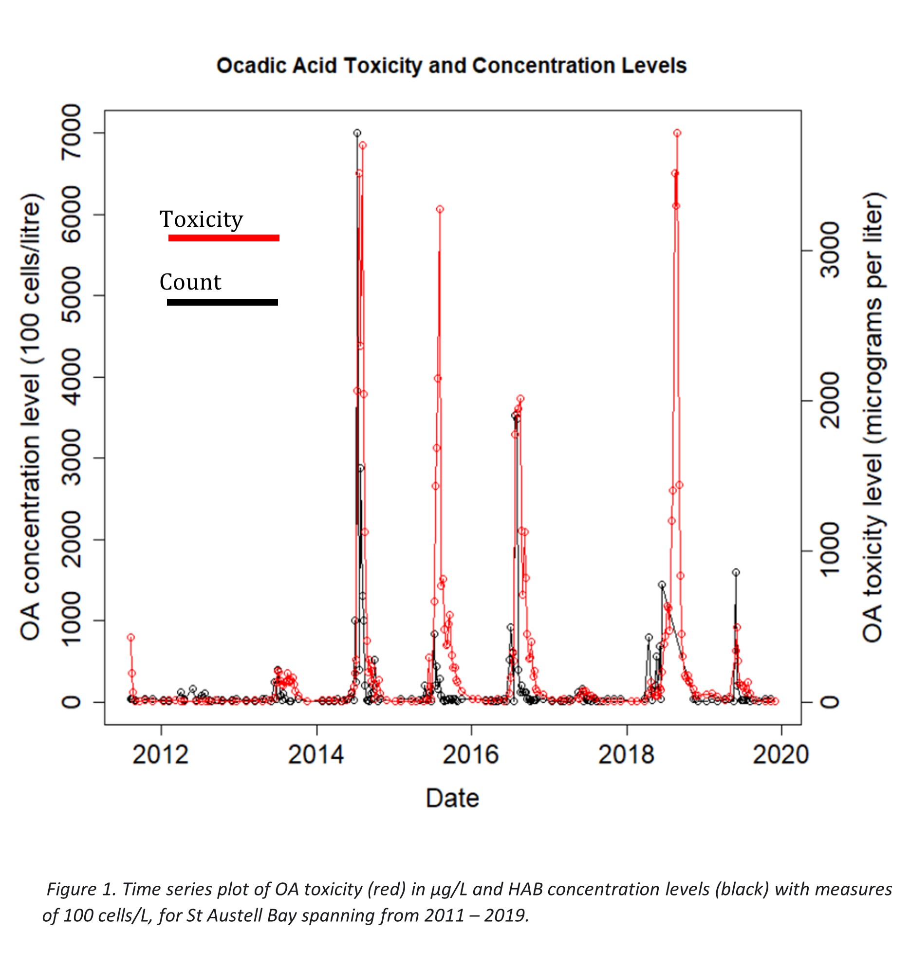
From the initial plot it is observed that the concentration levels do not coincide with the toxicity levels exactly, and this is because the concentration of HABs may be high, but they can be non-toxic in some cases. However, there is a very strong relationship between the two, where the concentration of HAB rises, the toxicity levels rise with it. And once the concentration starts to fall, the toxicity levels continue rising for some time and start to fall down only after some period of time. This indicates that the lagged concentration counts can be used as a variable for OA toxicity predictions. In order to measure this relationship, the cross-correlation (cross-covariance) function was applied between the two variables.
Table 3. Cross-correlation table for St Austell Bay between HAB cell count and OA toxicity measures showing cross-correlation for lags of -4 to 2
| Lag | -4 | -3 | -2 | -1 | 0 | 1 | 2 |
|---|---|---|---|---|---|---|---|
| St Austell Bay Correlation | 0.32 | 0.50 | 0.45 | 0.55 | 0.42 | 0.23 | 0.11 |
The result suggests that the strongest correlation occurs during the first negative lag. Meaning that the previous observation of HAB cell count correlates stronger with OA toxicity than the HAB cell count measure taken on the same day as the OA toxicity measures. Table 3 outlines the cross-correlation for the OA toxicity and HAB cell counts measures. Each lag corresponds to approximately 1.1 - 2.3 weeks, hence using the cell count measure from 1.0 - 2.3 weeks in the past to measure the OA toxicity at the current time will yield higher predictive power when modelling forecasts.
The plotted data in figure 1 also suggests a strong seasonal cycle, where the HAB toxicity rises in the warmer months (except the anomaly year of 2017), and this is expected due to higher temperatures in the water and more sunlight for the algae to receive nutrients from, allowing for greater growth.
Individually for St Austell Bay the HAB cell abundance (count) has 190 observations, and HAB OA toxicity 193 observations. However, when synchronising the two datasets together by dates, the dimensions are reduced to 154 observations. To avoid loss of data points, a model that captures the historic pattern can be fitted to interpolate the HAB counts. This can create good estimates for the full range of dates, allowing to synchronise cell count data and OA toxicity data without losing any information. Hence a GAM model with a smooth function of time and a substantial number of knots (k=70 in this case) was fitted to interpolate the missing cell count data and yield all possible values for every day of the time series. This was then done for the two other locations data.
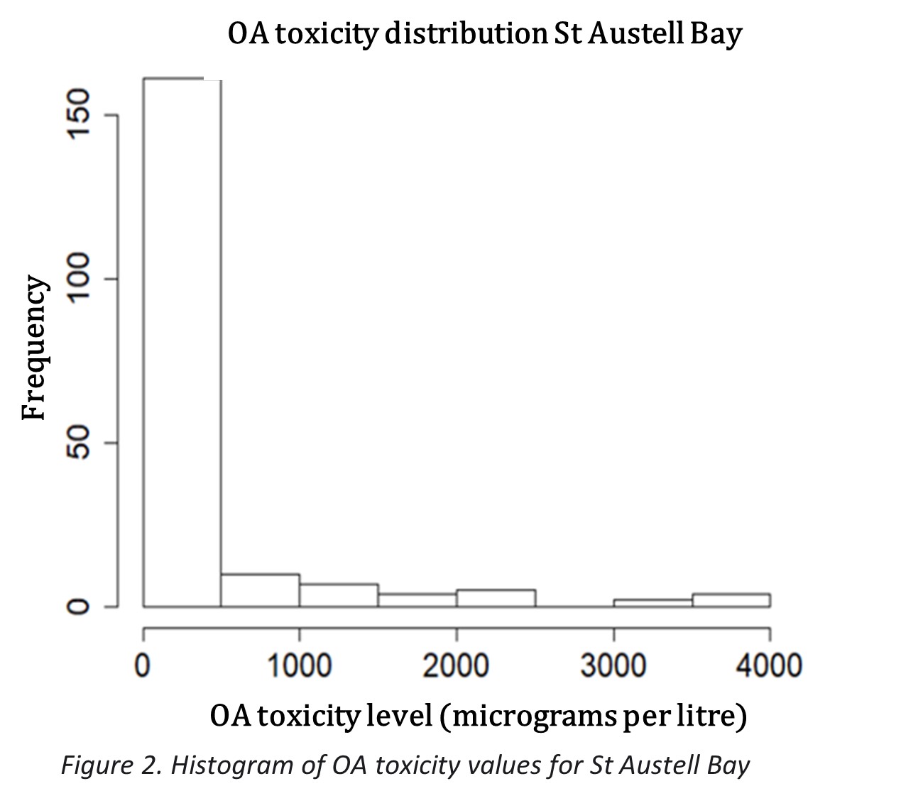
Recalling that the threshold limits for HAB cell abundance is 100 cells per litre, and threshold for OA toxicity is 160 mg/L, it will be important to take caution of the extreme high values for both measures in the data sets. Table 4 outlines summary statistics for the HAB cell abundance and OA toxicity, and shows the extreme high values of 7000 and 3700. Since the forecasting models' task is to warn when the toxicity breaches the threshold, such high values may potentially skew the predictions, so this aspect will need to be accounted for when building the models.
Table 4. Summary statistics for HAB cell abundance (count) as 100 cells per litre and OA toxicity (OA) as mg/L for St Austell Bay.
| Date | Count | OA | |
|---|---|---|---|
| Min | 2011-08-09 | 1.0 | 1.0 |
| Median | 2015-08-16 | 33.5 | 64.5 |
| Mean | 2015-08-08 | 227.5 | 309.6 |
| Max | 2019-12-03 | 7000.0 | 3700.0 |
Figure 2 shows the distribution of OA measures, where most values are below 500 mg/L and highlights the extreme high values.
Since the measurements are not taken on a consistent basis, it will be important to account for that when fitting any timer series models (e.g ARIMA) as well as when looking at any lags between HAB count and OA toxicity.
First steps of the project were to examine the findings of Schmidt W.'s paper[10], looking specifically at St. Austell and its respective OA toxicity levels. The same data sets were used to try and replicate the results. It is useful to introduce the location for better context, so that the results of the paper and the replicated models make sense.
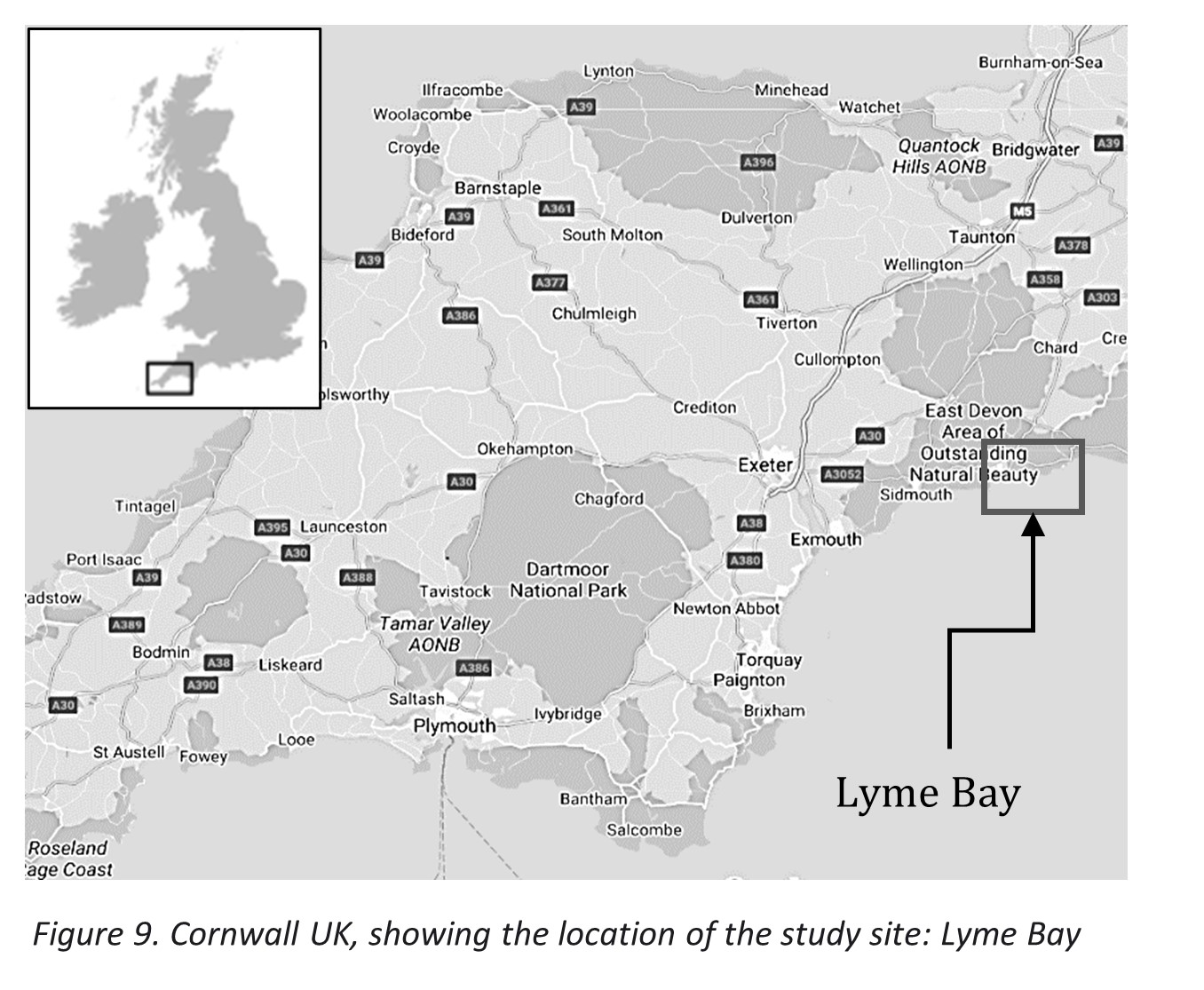
St Austell Bay
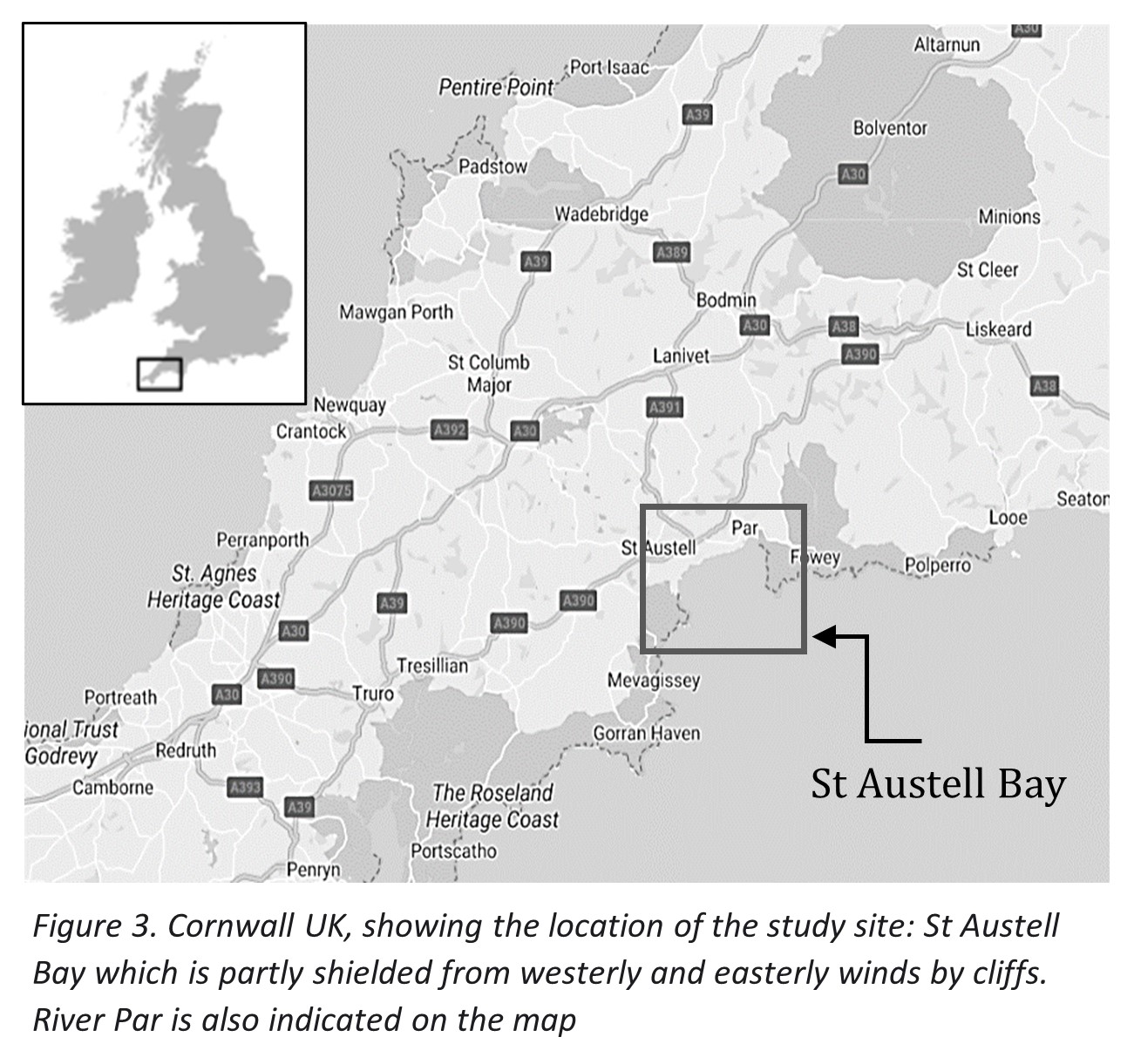
St Austell Bay is located on the south coast of Cornwall UK, covering an approximate area of 21 km3 and a mean depth of 5 m near the shore to 20 m at the mouth12. The bay includes 2 shellfish farms that harvest blue mussels. Main characteristics of the bay include small tidal current, the river 'Par' with other small streams that may influence near shore dynamics and cliffs shielding winds from the east. Taking note of the location's characteristics, the data sets with the environmental variables can now be looked at in detail. The main environmental variables (for which detailed information can be found in the original paper10) that span up to the end of 2018 to be looked at are the following:
- Rainfall & lagged rainfall (the rainfall on the day prior to OA sampling) – mm d-1
- River & lagged river flow rate – m s-1
- Wind speed –calculated from daily 10 m U wind and 10 m V wind instantaneous data at 00:00, 06:00, 12:00 and 18:00 h UTC
- Wind direction – same as wind speed
- Solar radiation (ssrd) - d-1
- Sea surface temperature (sst) - degrees Celsius
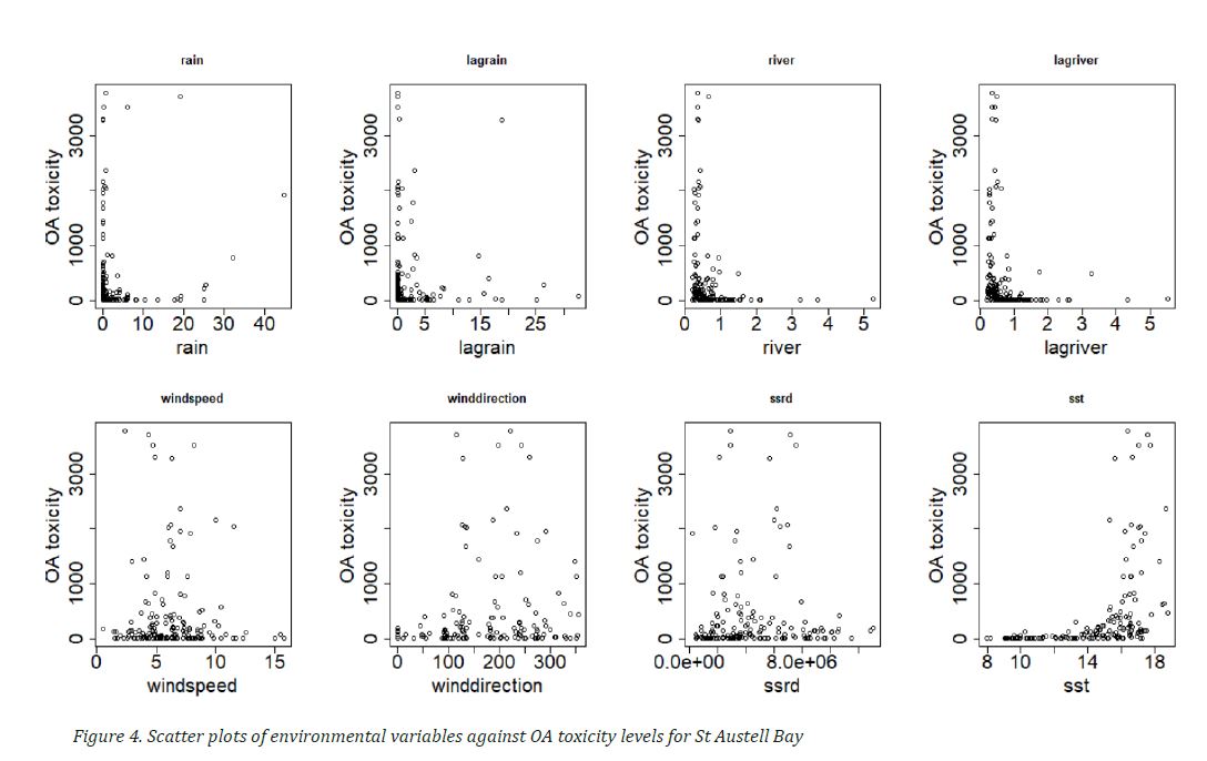
Initial data plots in figure 4 suggest that some variables have higher predictive power, such as the sea surface temperature and windspeed. And this can be confirmed when fitting a GAM of the following form:
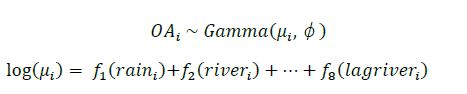
Where f is the smoothing function fitted to each variable. Due to the non-Gaussian nature of the response variable OA the GAM models are fitted with a log link function and a Gamma distribution. Initially all the environmental variables were set as smooth terms with knots equal to 4. The results of the model summary in table 5 and 6 below are in line with the results of Schmidt W's paper.
Table 5. p-values from the initial GAM model fitted to all environmental variables. An asterisk (*) marks variables that contributed significantly (p > 0.05) to the model
| VARIABLE | P-VALUE |
|---|---|
| rain. | 0.09 |
| river. | 0.08 |
| sea surface temperature (sst)*** | >2e-16 |
| wind direction. | 0.018 |
| wind speed* | 0.057 |
| solar radiation (ssrd) | 0.83 |
| lagriver | 0.34 |
| lagrain** | 0.00 |
Table 5 suggest that the most important variables for modelling OA toxicity are sea surface temperature, lagged rain, windspeed and wind direction.
Table 6. Significant Environmental variables from initial GAM model when including all parameters and Schmidt W’s paper GAM model.An asterisk (*) marks variables that contributed significantly (p > 0.05) to the model.
| Explanatory variables | |
|---|---|
| GAM0 | SST***, wind speed*, lag rain* |
| Schmidt W's GAM** 10 ** | ** SST *, solar radiation *, wind speed * and as smoothedterm: lag rainfall** |
Replicating the results of Schmidt W's Gam yielded similar but not exactly the same results, as the initial GAM was applied to an updated data set with more observations, as well as applying a smoothing term to all variables, as opposed to only some (e.g. lagged rainfall) in Schmidt W's GAM. Nevertheless, this preliminary GAM0 model is a suitable starting point.
This initial analysis is used to build the model further beyond the inclusion of only environmental variables. When plotting these variables as time series, it is evident that some of them follow a seasonal cycle, similar to the overall OA toxicity time series. This explains why the variable sea surface temperature (sst) is so significant in the initial GAM model since it correlates closely with the seasonal cycle and hence the response variable OA.
Main GAM models
The main GAM model that was developed incorporates the lagged HAB cell counts, a seasonal cycle (day of year) and a select few environmental variables that showed to have improved the overall model fit. The combined data set used has the following parameters outlined in table 7.
Table 7. Overview of the combined dataset used for training and evaluation of the GAM models for St Austell Bay.
| Training period | No. obs | Testing Period | No. obs |
|---|---|---|---|
| 2011-08-09 2018-07-24 | 155 | 2018-07-312018-08-28 | 5 |
As the aim is to develop a short-term forecasting model, the testing/evaluation period includes only 5 data points. This way the model is trying to predict approximately1-10 weeks in advance as every data point is calculated to be on average 2 weeks apart. A 2-week period would likely be the limit for accurate forecasting, which would give shellfish farmers a warning of possible OA threshold breaches (OA levels above 160 μg/L), therefore the first couple of predictions are to be considered with more importance than those further into the future. This would provide adequate amount of time to plan harvests and manage customer supply chains. However, the 2-week difference is an assumption based on the whole dataset, the difference between measurement intervals for the 5 evaluation data points is calculated to be a mean of 1-week for St Austell Bay. Which is more suited for the short-term forecasting challenge at hand than the averaged 2-week intervals.
Firstly the GAM (GAM1) model with the environmental variables and the seasonal trend is fitted to the data set and compared to a GAM (GAM2) model that is fitted to the time series of OA toxicity, for the same dates (same data set with 160 observations in table 7). Summary results for the most suitable GAMs (GAM1 and GAM2) are outlined in table 8.
Table 8. Summary of the most suitable GAM models for St Austell Bay. All variables are smoothed terms with knots set to 6 for GAM1 and 40 for the variable Time in GAM2 (to allow for capture of the historical time series). An asterisk (*) marks variables that contributed significantly (p > 0.05) to the model.
| variables | R2 | RMSE | AIC | |
|---|---|---|---|---|
| GAM1 | Lagged count***, day of year***, wind direction*, lag river | 0.53 | 1930 | 1819 |
| GAM2 | Time*** | 0.59 | 593 | 1703 |
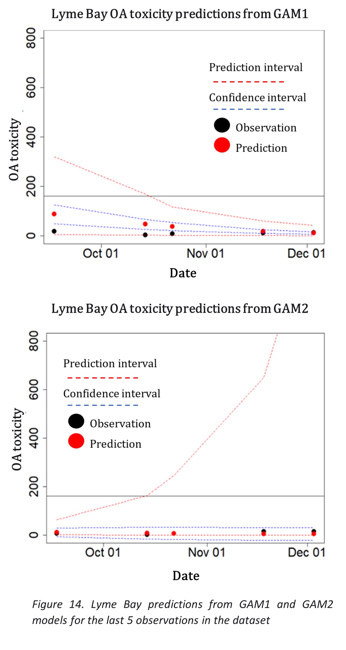
T he above model summaries are from the predictions of the last 5 observations using 155 observations for training. Comparing the time series GAM2 to the GAM1 it looks to be that the model based just on the time series is performing better, with a lower RMSE and AIC measures. However, when looking at the prediction intervals of the models, GAM1 captures the real observations better, especially for points further down the timeline, than GAM2. Hence the environmental variables and the structured seasonal cycle (day of year) play an important role in decreasing uncertainty for predictions. Figure 4 and 5 illustrates the difference in the prediction intervals of both models. GAM2 prediction intervals start to diverge to infinity down the timeline, whereas for GAM1 all of the observations are captured by the prediction intervals in a clearer manner. The figures also show that both models predict the first 2 observations much better than the subsequent 3 observations.
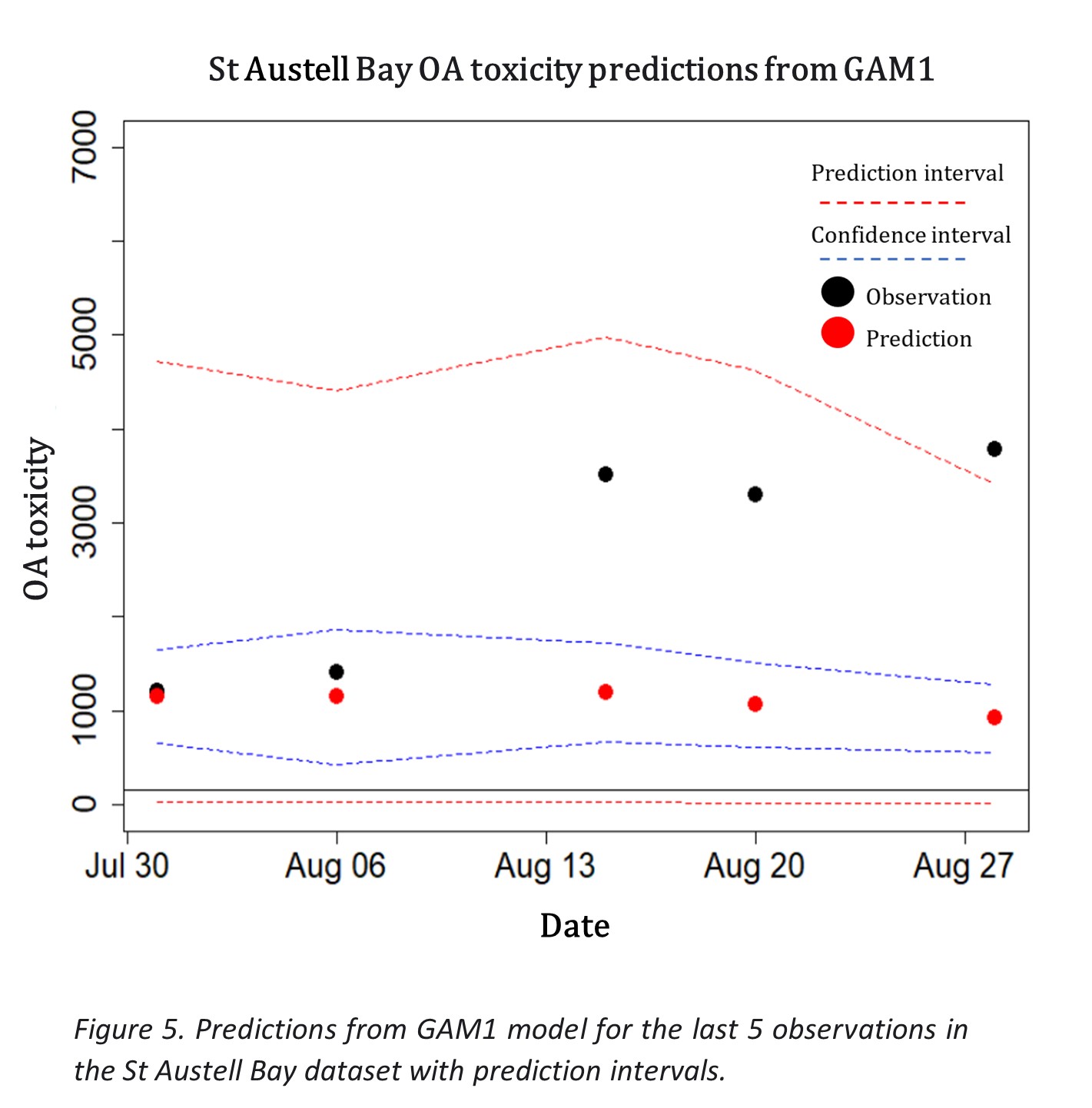
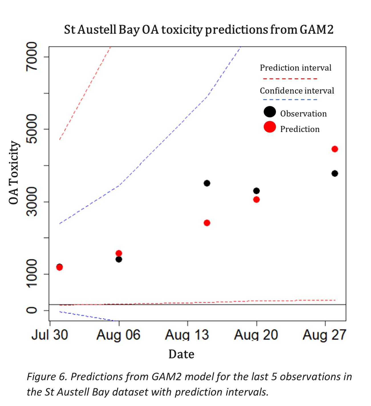
The approach of keeping the two models separate instead of adding the time variable to GAM1 was that when doing so, the overall model became overconfident. This yielded predictions with a higher RMSE score than when the two models are kept separate.
Rolling model retrain
It is also important to look at how the models predict across the time series, and not just for the last 5 observations of the data set. When both models undergo a retrain period, the overall trend in RMSE decreases as more observations are added to the training set. The way this was done, is by, first starting with 30 observations (50 for GAM2) and predicting the next 5 observations, subsequently adding the next observation to the training set, and again predicting the next 5, until all the data is used for training.
In addition to predicting the absolute values of the OA toxicity, it is also useful to predict the threshold breaches, on which the decision of farm closures is based. This approach will address the right skewness of the OA toxicity levels distribution (figure 2 as the extremely high values will no longer skew the predictions. The threshold at which the harvesting locations are closed is 160 μg/L of okadaic acid (OA). In order to see if the model predicted the closure of the shellfish farm (breached threshold), the OA toxicity levels are first converted into 1's if the level is above 160 and 0 if below the threshold. Adapting this approach to the last 5 predictions for GAM1 and GAM2, the results and accuracy scores are outlined in Table 10.
Table 10. True positives and true negatives for the developed GAM models. Number of observations to be predicted is 5.
| True positives | True negatives | Accuracy | |
|---|---|---|---|
| GAM1 | 5/5 | 0/0 | 100% |
| GAM2 | 5/5 | 0/0 | 100% |
The above true positives and true negatives are calculated for the predictions of the last 5 observations and only give insight into how the models are predicting for the time frame at the end of each data set. Both GAM models have shown to do a good job when predicting the threshold limits forecasted 1-10 weeks into the future (1 observation approximately equal to 2.2 weeks). The threshold breach is the base line for the decision making at the harvesting sites, whether to close or keep the farm open. As the number of observations used to predict the threshold is low, the accuracy is not entirely representative of how the model predicts across other time periods (e.g seasonal peaks). From the previous rolling-retrains (starting with 30-50 observations for training and adding 1 observation every re-train), the averaged accuracies are calculated in table 11.
Table 11. Averaged accuracy scores of the GAM models for threshold breaches, based on the rolling re-train.
| Accuracy | |
|---|---|
| GAM1 | 78% |
| GAM2 | 75% |
Table 11 suggests that the accuracy for any given time period when predicting the next 5 observations is slightly higher for GAM1, the model with lagged cell count and environmental variables, than the time series model GAM2. However, this is only a rough measure of the overall model accuracy. The method for calculating these figures is based on accuracy scores from each re trained model, meaning that each accuracy score is based on models with more data incrementally, and then averaged for the overall score. In addition to this the accuracy of the absolute OA toxicity value is higher for predictions of 1-2 weeks ahead compared to 10 weeks ahead, as seen previously in figures 4 and 5. Therefore, in theory, if these models are to be used, only the next predicted value should be taken into consideration until the model is retrained.
Lantivet and Lyme Bay
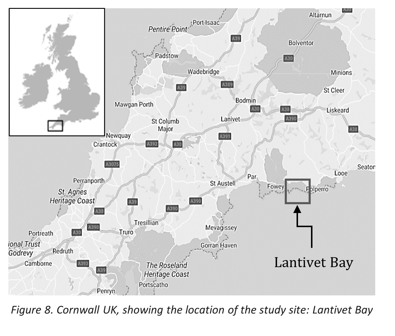
In this section, Lantivet Bay and Lyme Bay data will be analysed to see if the generic model approach used for St Austell Bay will yield similar results for these South West Coastal regions. Both Bays have different environmental characteristics to St Austell Bay, and are not shielded from eastern winds by the cliffs. The presence of rivers is also varied for both of these locations. Firstly, GAM1 and GAM2 will be applied to both locations to predict absolute OA values and subsequently the classification of threshold breaches will be predicted.
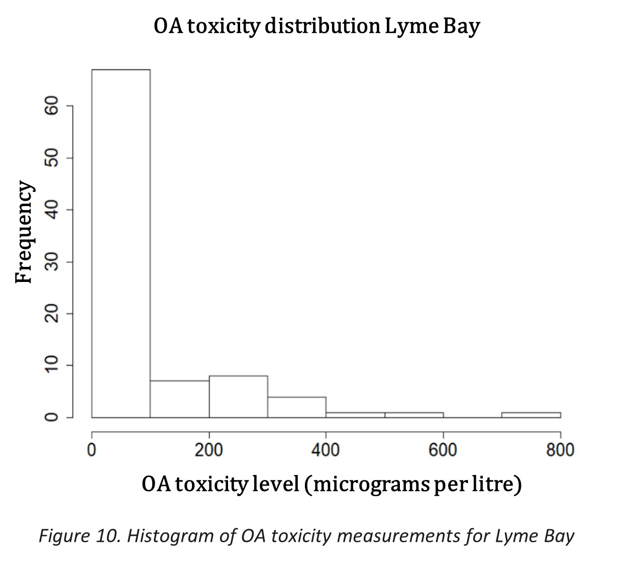
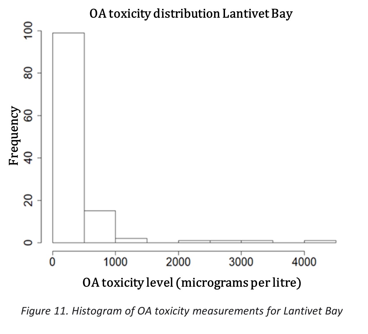
The histograms in figures 9 and 10 show the distribution of OA toxicity for both Bays. Both distributions are similar to that of St Austell Bay; however, Lyme Bay does not have such extreme values as St Austell and Lantivet Bays, with a maximum OA toxicity level of 800 compared to 4000 at Lantivet Bay and 7000 at St Austell Bay. Lyme Bay also has substantially less measurements that cross the threshold level of 160 mg/L, with overall less varied measurements.
The following figures 12 and 13 show the time series of the OA toxicity at each bay site, with the corresponding concentration levels. These figures show similar patterns to St Austell Bays time series, with the presence of a seasonal cycle with high toxicity in warmer months. However, the relationship between HAB cell count and toxicity levels for both bays differ from that of St Austell, in a way that indicates less lagged correlation, but still a strong relationship between the two.
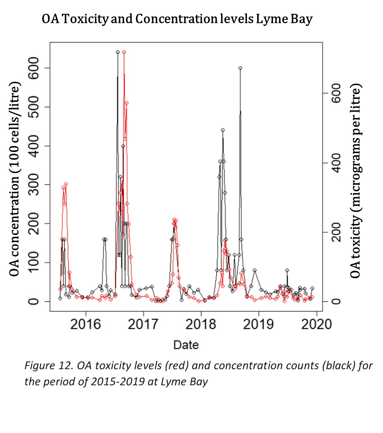
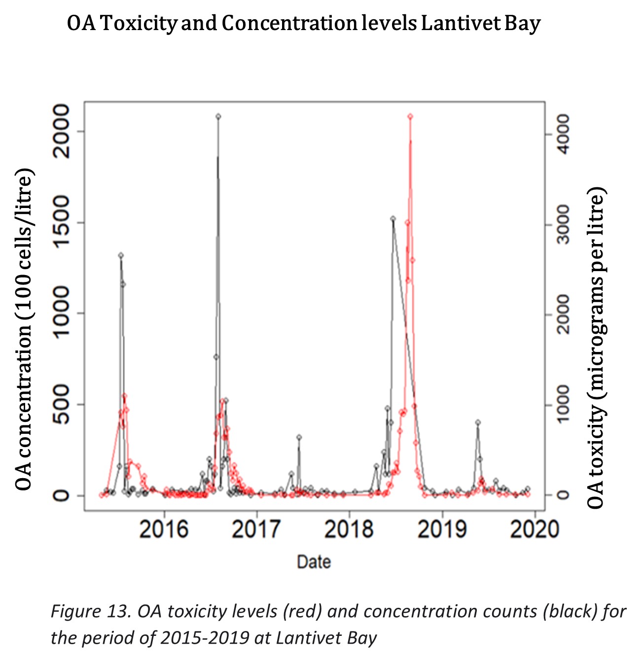
For Lyme Bay it looks as though the HAB cell count rises first, and after a period of time the OA toxicity starts rising. Lantivet Bay follows a pattern more similar to Lyme Bay than to St Austell Bay, with HAB cell count rising before OA toxicity, as opposed to both measures rising together as seen for St Austell in figure 1. Table 13 includes the cross-correlations for these two measures at Lyme bay and Lantivet bay.
Table 13. Cross-correlation table for Lyme Bay and Lantivet Bay between HAB cell count and OA toxicity measures, showing cross-correlation for lags of -4 to 2.
| Lag | -4 | -3 | -2 | -1 | 0 | 1 | 2 |
|---|---|---|---|---|---|---|---|
| Lyme Bay Correlation | 0.23 | 0.36 | 0.32 | 0.47 | 0.33 | 0.26 | 0.20 |
| Lantivet Bay Correlation | 0.40 | 0.40 | 0.45 | 0.39 | 0.34 | 0.22 | 0.10 |
The cross-correlation for all three bays is the lowest at lag zero if compared to the negative lags (up to fourth negative lag). GAM1 model uses the first negative lag as one of the predictors, for which St. Austell Bay had a correlation of 0.55, which is slightly higher than the first negative lags for Lyme and Lantivet Bay. Interestingly for Lantivet Bay, the correlation is higher for HAB cell counts that are collected further in the past, this may be due to more frequent collection intervals for this Bay (outlined in table 14). Yet still, the first negative lag has more correlation, hence more predictive power than the correlation at lag zero. This is a pattern seen in all three Bays.
Following on from the above it should also be noted that the mean difference in time periods between each measurement of OA toxicity for Lyme Bay is 2.56 weeks and for Lantivet Bay is 2 weeks. With Lantivet Bay having the most frequent intervals and Lyme Bay having the most consistent intervals. This is summarised for comparison in table 14.
Table 14. mean median maximum and minimum measures for the difference in OA toxicity collection dates in weeks for St Austell, Lyme and Lantivet Bays.
| Location | Mean | Median | Max | Min |
|---|---|---|---|---|
| St Austell Bay | 2.26 | 1.14 | 10.3 | 0.0 |
| Lyme Bay | 2.59 | 2.14 | 7.00 | 0.0 |
| Lantivet Bay | 2.00 | 1.00 | 15.9 | 0.6 |
Even with the differences in lagged HAB cell counts there are still similar patterns across the three Bays when looking at the time series plots. These similarities suggest that the models developed for St Austell Bay should produce similar results for these locations also.
The time periods for evaluation and testing are outlined in table 15 for each of the bays. The available data of OA toxicity and HAB cell count for both bays spans from 2015-2019, hence the time period for analysis is shorter and the number of total observations in also lower in comparison to St Austell Bay.
Table 15. Overview of the combined dataset used for the training and testing with the most suitable GAM model for Lantivet Bay and Lyme Bay.
| Bay | Training period | No. obs | Testing Period | No. obs |
|---|---|---|---|---|
| Lantivet Bay | 2015-07-22 2019-06-17 | 115 | 2019-07-162019-12-03 | 5 |
| Lyme Bay | 2015-07-22 2019-09-02 | 84 | 2019-09-172019-12-03 | 5 |
Although it is ideal to compare the bays when fitting the model to the same variables, the environmental variables data sets for Lative Bay and Lyme bay differ in structure to St Austell Bay and hence were not used. The model GAM1 still includes the lagged cell count and a seasonal component but omits the wind direction and lagged rain variables. The model setups are outlined in table 16 and 17 for both bays.
Table 16. Summary of the most suitable GAM models for _Lyme _Bay. All variables are smoothed terms with knots set to 6 for GAM1 and 45 for the variable Time in GAM2 (to allow for capturing the historical time series).
| variables | R2 | RMSE | AIC | |
|---|---|---|---|---|
| GAM1 | Lagged count***, Day of year*** | 0.54 | 39 | 835 |
| GAM2 | Time*** | 0.75 | 6 | 786 |
Table 17. Summary of the most suitable GAM models for _Lantivet_Bay. All variables are smoothed terms with knots set to 6 for GAM1 and 45 for the variable Time in GAM2 (to allow for capturing the historical time series).
| Variables | R2 | RMSE | AIC | |
|---|---|---|---|---|
| GAM1 | Lagged count***, Day of year*** | 0.56 | 297 | 1273 |
| GAM2 | Time*** | 0.88 | 28 | 1174 |
Classification of threshold breaches for the last 5 evaluated observations is outlined in table 18 below.
Table 18. True positives and true negatives for the developed GAM models for Lyme and Lantivet Bays. Number of observations to predict is 5 in every case.
| Model - Location | True positives | True negatives | Accuracy |
|---|---|---|---|
| GAM1 – Lyme | 5/5 | 0/0 | 100% |
| GAM2 – Lyme | 5/5 | 0/0 | 100% |
| GAM1 – Lantivet | 0/0 | 2/5 | 40% |
| GAM2 – Lantivet | 0/0 | 5/5 | 100% |
In the case of Lantivet Bay, the RMSE score for the predictions of absolute OA measures are smaller than that of St Austell Bays model, however the accuracy for classification of threshold breaches of GAM1 model is quite low, 40%. These metrics however must be taken with caution because the last few observations that were being tested were all very low values (3-74 μg/L ) shown in figure 15, for which the previous values in the training data set where comparatively higher. Since GAM1 is based on a seasonal cycle trend, it could in some cases skew the predictions for warmer months, which could be a possible explanation for the poor predictions at Lantivet bay. Figure 15 shows high predictions for month of August – September. This can be considered a sensitive area where the model will have difficulty correctly classifying the predictions, and would need to be cross checked with the predictions of the absolute OA values to see by how much they diverge from the threshold, and hence a decision would need to be made based on both pieces of information.
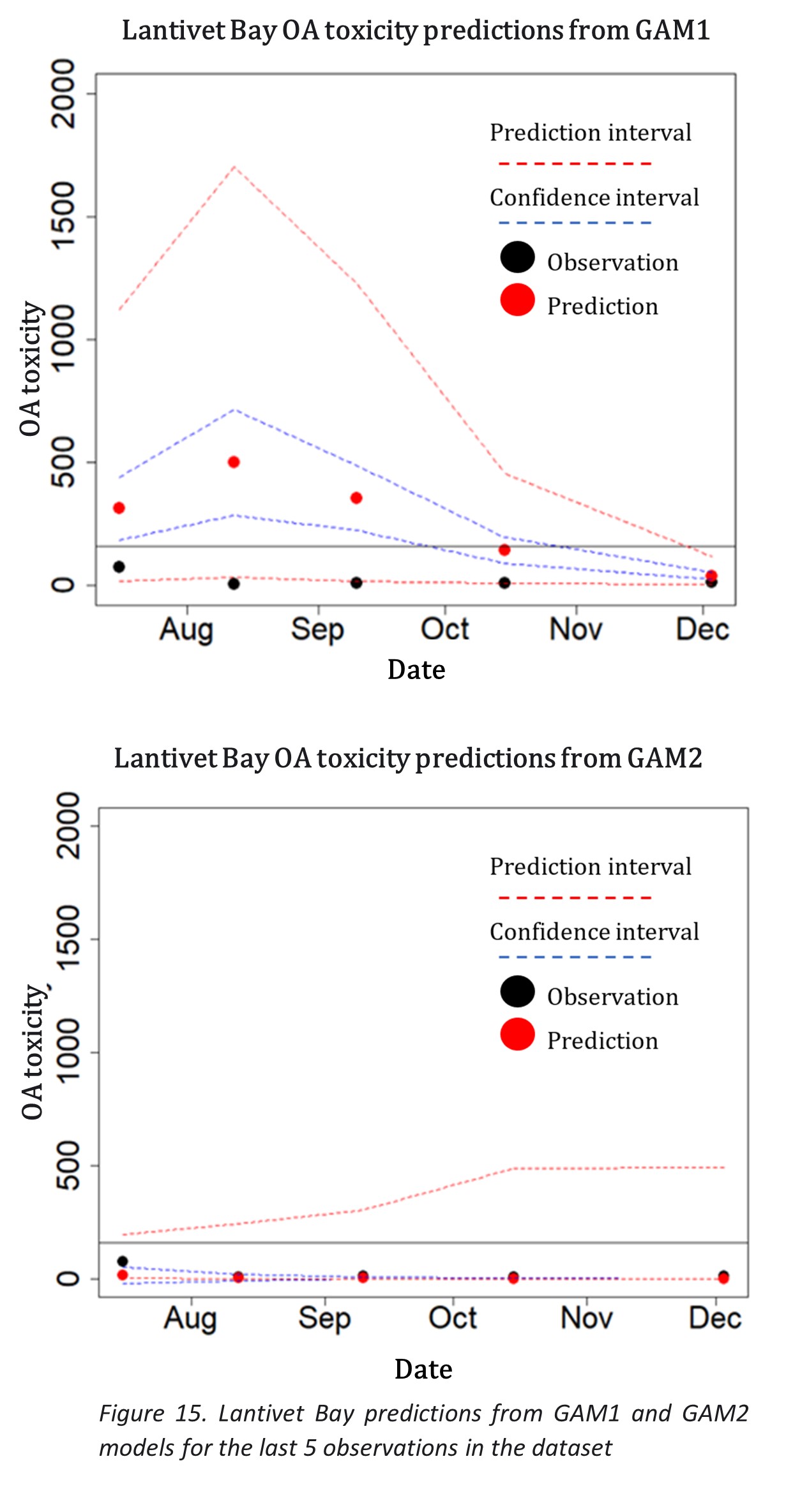
GAM2 for Lantivet Bay however predicted the absolute values and threshold breach classifications much better in comparison to GAM1.
Averaged classification of OA toxicity threshold breaches based on rolling-retrains of the models are outlined in the following table 19.
Table 19. Averaged accuracy scores of the GAM models for threshold breaches, based on the rolling re-train.
| Model - Location | Averaged accuracy |
|---|---|
| GAM1 – Lyme | 76% |
| GAM2 – Lyme | 79% |
| GAM1 – Lantivet | 84% |
| GAM2 – Lantivet | 82% |
Even without the additional environmental variables that help reduce the prediction intervals, the overall averaged accuracy scores for both models GAM1 and GAM2 are similar to the obtained results for St Austell Bay.
SUMMARY AND DICSUSSION
The statistical methods used in this project have shown that they are capable of producing short term forecasting solutions for the three investigated harvesting bays. And potentially adapted to more coastal locations across the South West of England. The GAM framework has demonstrated its ease of use when applied to in regard to OA toxicity. The smooth functions of GAMs allow for flexibility and addition of seasonal cycles that will adapt to the data for each location and capture the historic patterns.The models do not require lots of complex input variables to produce feasible results and deliver similar outputs across all bays even with different time scales of OA measurements and location characteristics. Data sets with 84 observations and with 160 observations have shown to be adequate. Having a few years' worth of data that captures seasonal changes is sufficient. Also, the modelling approach does not require heavy fine-tuning to suit the requirements of individual locations. Main advantages of this modelling approach are the use of readily available data, where HAB cell count and OA toxicity measures alone are able to produce feasible results. The addition of environmental variables (satellite observations and meteorological nowcasts and forecasts), which are also readily available in most cases, decrease the uncertainty of predictions when forecasting absolute OA toxicity values. The addition of these meteorological variables (windspeed, lagged rain) was only tested on St Austell Bay, however the models for Lyme Bay and Lantivet Bay still produced feasible results (with the exception of Lantivet Bay GAM1 model).As opposed to process-based models, the statistical approaches used in this project are much lighter in terms of computational power and these models can be easily and quickly adapted for shellfish farm management. Although the predictions of the absolute values of OA were not perfect, they were close to the original observations, yielding 100% accuracy for the threshold breaches classification on the 5 last observation for all three bays. The overall classification accuracy for GAM1 was 78% and for GAM2 was 75% when tested on St Austell Bay, and similar results for Lyme and Lantivet Bays (table 19).
Comparing the two approaches of GAM1 and GAM2 models, has shown that although GAM2 can be unstable (spikes in RMSE scores across rolling re-train) it has still predicted the classification breaches with 100% accuracy for all three bays, and had lower RMSE scores for the absolute OA values. GAM1 on the other hand has an advantage when capturing the real observations with its prediction intervals. Both approaches however produced similar averaged accuracy scores for the classification of threshold breaches.
However, there are still a number of limitations to that need to be discussed. Some limitations of the modeling approach performed in this project need to be addressed and possibly lead to further development and research in the field of HAB toxicity forecasting. Although the OA toxicity levels are seasonal which creates a good predictive pattern, there are still years with high spikes and years with no spikes at all during the warmer months where one would expect to have high levels of OA. This is a limitation of the statistical approach as mentioned earlier from the lakes model study [8]. If the underlying ecological conditions change, the model will not have enough historical data on these new conditions to create predictive patterns and would need some time to re-adapt. Additionally, most of the analysis for accuracy was performed on the last 5 observations of the data sets, which is only a snippet of the whole OA toxicity time series. Although a rolling re-train was performed to assess how the models would predict at any point in the OA time series, and hence yield accuracy scores for the threshold breaches, the method is still limited by averaging across the re-trained models. This means the accuracy scores are not taking into account that the model is performing on average better with every retrain, as more data is being introduced, but averaged across all models. More weighting should be applied to models further down the re-train period that have more data. Further limitation is the use of datasets that span until different end dates. This was mostly a problem for St Austell Bay, as the environmental variables data set only spanned until 2018, where the OA toxicity and HAB cell count data were collected up to the end of 2019, giving insight into a whole additional seasonal cycle. Ideally it would be good to compare GAM1 and GAM2 models on the very recent data. In contrast the data for Lantivet and Lyme Bay did span up to end of 2019 but had shorter time series, starting in 2015 as opposed to 2011 for St Austell Bay. Although more recent data is of more importance, having additional historic data would be beneficial, especially for fairer model comparison between the three bays. Another limitation is the inconsistent collection intervals of OA toxicity and HAB cell counts, where the difference spans from 1-15 weeks in between collection dates. This limits the approaches that can be used for modelling the time series of OA toxicity, for example an ARIMA (Autoregressive Integrated Moving Average) model would require consistent intervals for forecasting and hence could not be applied to the data at hand. In addition, these inconsistencies in measurement intervals limit the use of the lagged cell count variables, since the cross-correlation measures the relationship between arbitrary time intervals, one lag cannot be equated to a specific time frame. Hence the model is only using HAB cell counts lagged by one previous value and assuming it is on average 2-weeks in the past. Whereas if the measurements were to be consistent, the lagged HAB cell counts could have been investigated further as an additional variable including taking the mean of the 4 previous lags which would yield a variable with high predicative power. This was attempted in early staged of the project, but later disregarded due to not knowing the specific time intervals between each lag. However, there is a clear relationship between lagged HAB cell counts and the OA toxicity, and further research in this area would be beneficial.
CONCLUSION
In conclusion the modeling approach has shown to produce feasible results that could be adapted into a useful tool for shellfish farm decision making. Both models (GAM1 environmental model and GAM2 time series model) demonstrated promising abilities for short-term forecasting. The approach was shown to be easily adapted to multiple bays around South West England. Comparing three bays with the general approach has yielded promising results, but with fine tuning can be further improved for each specific location.
REFERENCES
-
Council B. Aquaculture - BBSRC [Internet]. Bbsrc.ukri.org. 2020 [Accessed 8 September 2020]. Available from: https://bbsrc.ukri.org/research/food-security/aquaculture/
-
Biotoxin and phytoplankton monitoring [Internet]. Food Standards Agency. 2020 [Accessed 31 July 2020]. Available from: https://www.food.gov.uk/business-guidance/biotoxin-and-phytoplankton-monitoring
-
Lucas JS, Southgate PC (2012) Aquaculture: farming aquatic animals and plants. Wiley-Blackwell, West Sussex
-
Marine Environments, Harmful Algal Blooms, CDC [Internet]. Cdc.gov. 2020 [Accessed 31 July 2020]. Available from: https://www.cdc.gov/habs/illness-symptoms-marine.html
-
Public Datastes [Internet]. ECMWF. 2020. [Accessed 31 July 2020]. Available from: https://apps.ecmwf.int/datasets/
-
UK Enviroment Agency rain and river data, provided by the College of Life and Environmental Sciences of University of Exeter
-
ERSEM - Plymouth Marine Laboratory [Internet]. Pml.ac.uk. 2020 [Accessed 31 July 2020]. Available from: https://www.pml.ac.uk/Modelling_at_PML/Models/ERSEM
-
Chaffin J, Linking Models and Field Experiments to Forecast Algal Bloom Toxicity in Lake Erie - NCCOS Coastal Science Website [Internet]. NCCOS Coastal Science Website. 2020 [Accessed 1 August 2020]. Available from: https://coastalscience.noaa.gov/project/linking-models-field-experiments-forecast-algal-bloom-toxicity-lake-erie/
-
Janssen A, Janse J, Beusen A, Chang M, Harrison J, Huttunen I et al. How to model algal blooms in any lake on earth. Current Opinion in Environmental Sustainability. 2019;36:1-10.
-
Schmidt W, Evers-King H, Campos C, Jones D, Miller P, Davidson K et al. A generic approach for the development of short-term predictions of Escherichia coli and biotoxins in shellfish. Aquaculture Environment Interactions. 2018;10:173-185.
-
Campos, C.J.A., Kershaw, S.R. & Lee, R.J. Environmental Influences on Faecal Indicator Organisms in Coastal Waters and Their Accumulation in Bivalve Shellfish. Estuaries and Coasts 36, 834–853 (2013). https://doi.org/10.1007/s12237-013-9599-y
-
Sherwin T, Jonas P. The impact of ambient stratification on marine outfall studies in British waters. Marine Pollution Bulletin. 1994;28(9):527-533.